DRYP Tutorial
Runing the Tilted-V catchment model test
This folder contains files to run the tilted-V catchment model.
Model parameters and simulation settings
The model requires a series of files that correspond to the parameter of the model. The parameters files have to be specified in the model input file: input_test.dmp
The model also requires a setting file where all the model simulation parameters are specified: setting_test.dmp
The example files are all provided in this directory for you to modify or replace, more information on the details of parameters and creating the DRYP inputs can be found here.
Running the simulation
Before you run the model, it is recommended to follow the steps for installation found here and activate the conda environments created for you in the instillation using this command:
conda activate cwld
Once all model and simulation parameters have been specified, the model can be run.
To run the test model, the test_dryp.py have to be used. This contains the path of the model input file, input_test.dmp.
If the model output matches the expected results provided in the /output_test/ folder, the test will result in no assertion errors.
The test can can also be run from the python command line or a python file with the following code:
from cuwalid.dryp.main_DRYP import run_DRYP

run_DRYP("test_input/input_test.json")
The location of all file locations must be relative to the location you run the file from. This example has the input in a directory called ‘test_input’ in the main directory
Model outputs
The model outputs from the test function should be similar to the figure below:
The figure shows the main hydrological fluxes obtained as a result of the precipitation and potential evapotranspiration used as a forcing dataset.
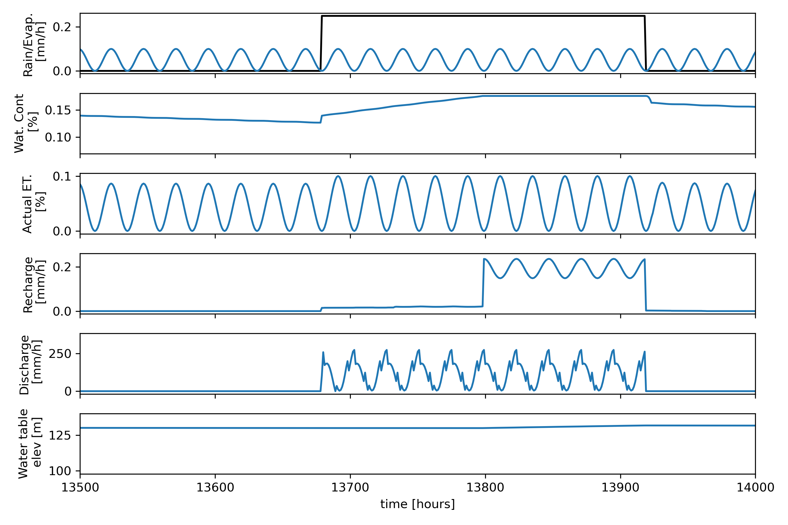
Model results show how average fluxes over the catchment vary in relation to the precipitation (first panel, backline). It is expected that precipitation increases the water content of the soil, but due to evapotranspiration losses, the amount of water available in the soil will be reduced at rates proportional to the available water content.
Rates of actual evapotranspiration vary depending on the availability of water, if there is enough water in the soil, water will be lost at potential rates (first panel blue line). if there is no water available the rate will be zero.
If the soil storage capacity of the soil is reached, water will percolate to the groundwater reservoir and produce recharge (fourth panel), this will in turn increase the water table elevation (bottom panel).
Running a regional model
DRYP was designed to perform hydrological simulations at large or hyper resolution hydrological models, so a version a regional scale model for the Horn of Africa Dryland region has been developed. This model is still on going further development, however, a first version of this model is availble at .
Running the large scale model may need additional computation resources to speed up the running process. This model has been set up for HPC server, however, a short version of the model can be prepared and executed using the DRYP pre-processing tools, assuming that all parameters maps are provided.
Creating a hydrological model from regional datasets
Discharge stored in the ‘avg’ file corresponds to the first row of the coordinate file. Therefore, in order to close the mass balance of the catchment, the first row of the coordinate file must be the coordinate of the catchment output.
Finally, an example of input parameter file is shown bellow, user can copy this template to create a nuew model.
Any values shown as null can be excluded from the json (defaults will be used), this example is just to present all the possible variables that could be used. In addition, variables labelled “required” must be given to run the DRYP model. Any other variables shown to have a value are showing the default parameters that will be used.
  1{
  2
  3    "model_name": "DRYP_model_sim",
  4    "path_input": "",
  5
  6    "TERRAIN": {
  7       "path_dem": "required",
  8       "path_Qo": null,
  9       "path_fdl": null,
 10       "path_riv_decay": null,
 11       "path_mask": null,
 12       "path_riv_len": null,
 13       "path_riv_width": null,
 14       "path_riv_elev": null,
 15       "path_of_bc_flux": null
 16    },
 17
 18    "VEGETATION": {
 19       "path_veg_kc": null,
 20       "path_veg_lulc": null
 21    },
 22
 23    "UNSATURATED": {
 24       "path_uz_theta_sat": null,
 25       "path_uz_theta_res": null,
 26       "path_uz_theta_awc": null,
 27       "path_uz_theta_wp": null,
 28       "path_uz_rootdepth": null,
 29       "path_uz_lambda": null,
 30       "path_uz_psi": null,
 31       "path_uz_ksat": null,
 32       "path_uz_sigmaksat": null,
 33       "path_uz_theta": null,
 34       "path_riv_ksat": null,
 35       "path_uz_bottomksat": null,
 36       "path_uz_bc_flux": null
 37    },
 38
 39    "SATURATED": {
 40       "path_sz_mask": null,
 41       "path_sz_ksat": null,
 42       "path_sz_sy": null,
 43       "path_sz_wte": null,
 44       "path_sz_bc_flux": null,
 45       "path_sz_bc_head": null,
 46       "path_sz_bottom": null,
 47       "path_sz_depth": null,
 48       "path_sz_bdd": null,
 49       "path_sz_type": null
 50    },
 51
 52    "METEO": {
 53       "path_pre": null,
 54       "path_pet": null,
 55       "path_aof": null,
 56       "path_lai": null,
 57		 "path_savi": null,
 58		 "path_kc": null,
 59   	 "path_TSOF": null,
 60   	 "path_TSUZ": null,
 61   	 "path_TSSZ": null,
 62   	 "path_TSav": null
 63    },
 64
 65    "OUTPUT": {
 66       "path_out_sz": null,
 67       "path_out_uz": null,
 68       "path_out_oz": null,
 69       "path_output": null,
 70       "path_setting": null,
 71       "path_store_settings": null
 72    },
 73
 74    "RIPARIAN": {
 75       "path_rp_theta_sat": null,
 76       "path_rp_theta_res": null,
 77       "path_rp_theta_awc": null,
 78       "path_rp_theta_wp": null,
 79       "path_rp_rootdepth": null,
 80       "path_rp_lambdas": null,
 81       "path_rp_psi": null,
 82       "path_rp_ksat": null,
 83       "path_rp_sigmaksat": null,
 84       "path_rp_theta": null,
 85       "path_rp_width": null
 86    },
 87
 88    "INTERCEPTION": {
 89       "path_veg_lulc_frac": null,
 90       "path_veg_hs_savi": null,
 91       "path_veg_hs_par_a": null,
 92       "path_veg_hs_par_b": null,
 93       "path_veg_hs_savi_min": null,
 94       "path_veg_hs_savi_max": null,
 95       "path_veg_hs_lai": null,
 96       "path_veg_hs_tap_depth": null,
 97       "path_veg_hs_extinction_depth": null,
 98       "path_veg_rp_par_a": null,
 99       "path_veg_rp_par_b": null,
100       "path_veg_rp_savi_min": null,
101       "path_veg_rp_savi_max": null,
102       "path_veg_rp_lai": null,
103       "path_veg_rp_tap_depth": null,
104       "path_veg_rp_extinction_depth": null,
105       "path_veg_rp_fcw": null,
106       "path_veg_rp_sca": null
107    },
108    "WATER_BODIES": {
109      "path_lake_depth": null,
110      "path_pnd_hmax": null,
111      "path_pnd_Amax": null,
112      "path_pnd_Vo": null
113   }
114 }
Information about simulation parameters such as period or time step must be provided in a json. This file contains parameters that control the simulations such as simulation period, format of input files as well as the activation of model components such as groundwater flow.
Information related to simulation period should be specified as the initial and final date of the simulation. Date must be specified as integers separated by spaces (e.g. 2001 1 9), zeros on the left side are not allowed (e.g 2001 01 19, will raise an error).
Time has to be specified in minutes, with a maximum time step of one day (1440 min). Time step must be an integer, and values must be rational fraction of the hour (e.g 20 min is allowed but 25 will stop the simulation) when sub-hourly time step is set. In case of hourly time steps, it must be a rational fraction of the day (e.g. 180 min (3h) is allowed but 300 min (5h) will result in errors). The time step of the groundwater components can not be less than the surface component.
The format of precipitation, evapotranspiration, vegetation, boundary conditions are shown below respectively:
csv file (only one file, that will be applied to the whole model domain)
netCDF file, only when one file is provided for the entire simulation period.
netCDF files, when yearly files are provided
netCDF files, when monthly fiels are provided
netCDF files, for DAILY netCDF files
netCDF files, for ensamble netCDF files (only for STORM)
The time frequency of the of model should be in minutes as time units. Note that it is not the time step of the model, it is only of the forcing dataset.
The model also accept datasets that are not in the model grid projection, or do not have the same grid size. For those cases, we can specified if each dataset requires a reprojection and/or interpolation. These options can be activated by changing the value from 0 to 1 on each of the corresponding dataset values for reprojection and interpolation, respectively. The order of the reading iptions parameters is not allowed to change, it will result in errors or even stop the simulation.
The following is an example of the configuration of reading parameters options.
"READING": {
    "data_reading": {
        "pre": 0,
        "pet": 0,
        "abs": 0,
        "kc": 0,
        "flux": 0,
        "savi": 0,
        "savi_min": 0,
        "savi_max": 0
        },
    "data_step": {
        "pre": 60,
        "pet": 60,
        "abs": 60,
        "kc": 60,
        "flux": 60,
        "savi": 60,
        "savi_min": 60,
        "savi_max": 60
        },
    "data_reproject": {
        "pre": true,
        "pet": true,
        "abs": true,
        "kc": true,
        "flux": true,
        "savi": true,
        "savi_min": true,
        "savi_max": true
        },
    "data_interp": {
        "pre": true,
        "pet": true,
        "abs": true,
        "kc": true,
        "flux": true,
        "savi": true,
        "savi_min": true,
        "savi_max": true
        }
},
DRYP has four types of infiltration methods implemented. The following codes can be chosen depending on the infiltration approach adopted:
Schaake model,
Philip’s equation,
Upscaled Green and Ampt,
Modified Green and Ampt method.
For the groundwater component, three different approaches for groundwater flow conditions are available:
Constant transmissivity,
Variable transmissivity with depth, fully unconfined conditions,
Transmissivity function,
Multi-aquifer settingd, it will enable the use of multiple aquifer types domains (a file must be provided).
The groundwater components can be activated or disabled, a value of 1 enable the groundwater component whereas a value of 0 disables it. A value of 2 will activate a two layer groundwater component (this component is still being tested).
The groundwater approach is specified along with the activation code of the groundwater component as shown in the example below (not required for the two-layer model):
Run Groundwater - Type: 0-Cons 1-Unc 2-func 3-Multi
1 1
In case that the approach is not specified, the “variable transmissivity”, option 0, is used as default approach.
To save model results as netCDF files change the boolean (true/false) under ‘OUTPUT’. Line “output_dt” is used to specify the aggregation frequency. Frequency should be specified as integer and a string character. Accepted character are D for days, M for months and Y for years, an example is specified below:
"output_grid": true,
"output_dt": "1H",
A set of parameters that globally modify the model parameters are also specified in the simulation settings file. Values are scale factors of the following parameters, this values are unitless:
kdt, for water partitioning of the Shaake infiltration approach,
kDroot, for rooting depth,
kAWC, for available water content,
kKsat for the saturated hydraulic conductivity of the soil,
kSigma, for the standard deviation of the saturated hydraulic conductivity of the Modified Green and Ampt approach,
kKch, for infiltration rates in the channel,
kT for decay parameter of discharge,
kKaq for aquifer saturated hydraulic conductivity,
kSy for aquifer specific yield factor,
  1{
  2  "SIMULATION_PERIOD": {
  3      "start_date": "2000 1 1",
  4      "end_date": "2002 1 3"
  5  },
  6
  7  "PROJECTION" : null,
  8
  9  "TIMESTEP_SETTINGS": {
 10      "dt_of": 60,
 11      "dt_uz": 60,
 12      "dt_gw": 60
 13  },
 14
 15  "READING": {
 16
 17      "data_reading": {
 18          "pre": 0,
 19          "pet": 0,
 20          "abs": 0,
 21          "kc": 0,
 22          "fluxOF": 0,
 23          "fluxUZ": 0,
 24          "fluxSZ": 0,
 25          "savi": 0,
 26          "savi_min": 0,
 27          "savi_max": 0,
 28          "lai": 0,
 29          "av": 0
 30          },
 31      "data_step": {
 32          "pre": 60,
 33          "pet": 60,
 34          "abs": 60,
 35          "kc": 60,
 36          "fluxOF": 60,
 37          "fluxUZ": 60,
 38          "fluxSZ": 60,
 39          "savi": 60,
 40          "savi_min": 60,
 41          "savi_max": 60,
 42          "lai": 60,
 43          "av": 60
 44          },
 45      "data_reproject": {
 46          "pre": true,
 47          "pet": true,
 48          "abs": true,
 49          "kc": true,
 50          "fluxOF": false,
 51          "fluxUZ": false,
 52          "fluxSZ": false,
 53          "savi": true,
 54          "savi_min": true,
 55          "savi_max": true,
 56          "lai": true,
 57          "av": true
 58          },
 59      "data_interp": {
 60          "pre": true,
 61          "pet": true,
 62          "abs": true,
 63          "kc": true,
 64          "fluxOF": false,
 65          "fluxUZ": false,
 66          "fluxSZ": false,
 67          "savi": true,
 68          "savi_min": true,
 69          "savi_max": true,
 70          "lai": true,
 71          "av": true
 72          },
 73      "data_projection" : {
 74		  "pre": "EPSG:4326",
 75		  "pet": "EPSG:4326",
 76		  "abs": "EPSG:4326",
 77		  "kc": "EPSG:4326",
 78		  "fluxOF": "EPSG:4326",
 79		  "fluxUZ": "EPSG:4326",
 80		  "fluxSZ": "EPSG:4326",
 81		  "savi":"EPSG:4326",
 82		  "savi_min": "EPSG:4326",
 83          "savi_max": "EPSG:4326",
 84          "lai": "EPSG:4326",
 85          "av": "EPSG:4326"
 86          }
 87  },
 88
 89  "COMPONENTS": {
 90      "method_inf": 1,
 91      "run_gw": true,
 92      "method_gw": 0
 93  },
 94
 95  "OUTPUT": {
 96      "output_csv": true,
 97      "output_grid": false,
 98      "output_dt_csv": "1M",
 99      "output_dt": "1M"
100  },
101
102  "GLOBAL_FACTORS": {
103      "uz_kdt": 1.0,
104      "uz_kdroot": 1.0,
105      "uz_kawc": 1.0,
106      "uz_kkast": 1.0,
107      "uz_ksigma": 1.0,
108      "riv_kksat": 1.0,
109      "riv_kdecay": 1.0,
110      "riv_kwidth": 1.0,
111      "sz_kksat": 1.0,
112      "sz_ksy": 1.0,
113      "of_kflow": 1.0
114  }
115}
When datasets are not in the same projection system thatn the model domain (UTM), a projection settings file should ne provided. It should contain the projection system of model, and the projection system of each dataset. An example is presented below:
1PROJECTION
2Model
3+proj=laea +lat_0=5 +lon_0=20 +x_0=0 +y_0=0 +datum=WGS84 +units=m +no_defs
4Datasets:
5List projection on the order of settings file:
6EPSG:4326
7EPSG:4326
8EPSG:4326
This component is still under development
This component is still under development:
1OFBC
2Flux data for time variable boundary conditions ----(1)
3../DynaVeg/input/DV_OF_flux.csv
4List points or raster map if netCDF not provided ---(3):
5../DynaVeg/input/DV_flux_points.csv
6other ----------------------------------------------(5):
7none
8other ----------------------------------------------(7):
{"store_var_grid":{
'pre': True,
'pet': True,
'run': True,
'aet': True,
'inf': True,
'tht': True,
'rch': True,
'egw': True,
'wte': True,
'gdh': True,
'twsc': True,
'chb': True,
'tls': True,
},
"store_var_point":{
'aet': True,
'inf': True,
'dis': True,
'tht': True,
'rch': True,
'wte': True,
'gdh': True,
'ssz': True,
},
"store_var_avg": {
'pre': True,
'pet': True,
'run': True,
'aet': True,
'inf': True,
'tht': True,
'rch': True,
'egw': True,
'wte': True,
'gdh': True,
'twsc': True,
'chb': True,
'tls': True,
},
"store_ver_grid_rp": {
'aet': True,
'fch': True,
'tls': True,
'tht': True,
'ssz': True,
}
}